3. 建模与调参
3.1 载入数据
1 | import pandas as pd |
3.2 线性回归
1 | continuous_feature_names = [x for x in sample_feature.columns if x not in ['price','brand','model']] |
1 | # 将非数值型类型转换为数字型类型 |
1 | # 划分为特征向量和标签向量 |
使用sklearn简单建模
1 | from sklearn.linear_model import LinearRegression |
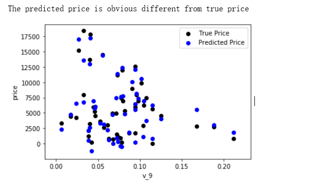
绘制特征v_9的值与标签的散点图,图片发现模型的预测结果(蓝色点)与真实标签(黑色点)的分布差异较大,且部分预测值出现了小于0的情况,说明我们的模型存在一些问题
1 | from matplotlib import pyplot as plt |
这是由于咱们在EDA就发现的情况,即price的分布存在长尾问题,所以我们对price进行log变换后再进行训练。
1 | train_y_ln = np.log(train_y+1) |
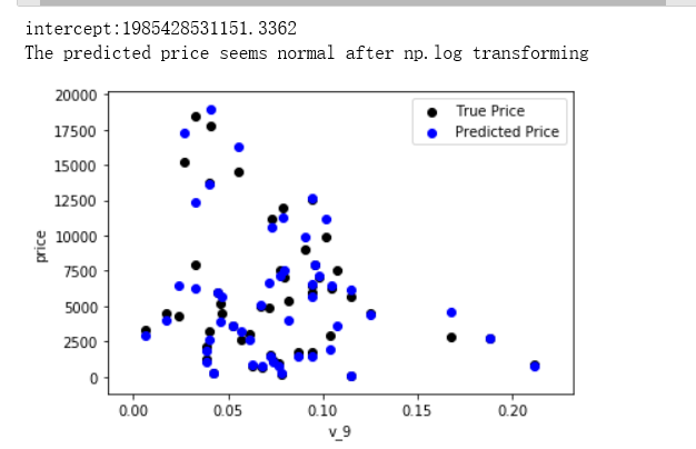
看起来,已经比上面那张图要好很多。
3.3 k折交叉验证
在使用训练集对参数进行训练的时候,经常会发现人们通常会将一整个训练集分为三个部分(比如mnist手写训练集)。一般分为:训练集(train_set),评估集(valid_set),测试集(test_set)这三个部分。这其实是为了保证训练效果而特意设置的。其中测试集很好理解,其实就是完全不参与训练的数据,仅仅用来观测测试效果的数据。而训练集和评估集则牵涉到下面的知识了。
因为在实际的训练中,训练的结果对于训练集的拟合程度通常还是挺好的(初始条件敏感),但是对于训练集之外的数据的拟合程度通常就不那么令人满意了。因此我们通常并不会把所有的数据集都拿来训练,而是分出一部分来(这一部分不参加训练)对训练集生成的参数进行测试,相对客观的判断这些参数对训练集之外的数据的符合程度。这种思想就称为交叉验证(Cross Validation)1 | %matplotlib inline |
3.4 嵌入式特征选择
嵌入式特征选择是将特征选择过程与学习器训练过程融为一体,两者在同一个优化过程中完成,即在学习器训练过程中自动地进行了特征选择。
1 | from sklearn.feature_selection import SelectFromModel |
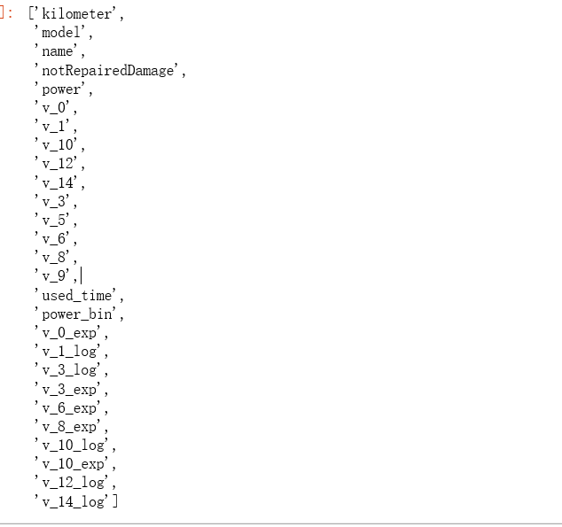
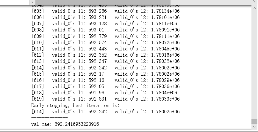
但是我用筛选出来地这27个特征重新做5折交叉验证,效果却比不做特征筛选地要差。
3.5 GridSearchCV 网格搜索调参
GridSearchCV:一种调参的方法,当你算法模型效果不是很好时,可以通过该方法来调整参数,通过循环遍历,尝试每一种参数组合,返回最好的得分值的参数组合。
1 | from sklearn.model_selection import GridSearchCV |

3.6 贝叶斯调参
贝叶斯调参:贝叶斯优化是一种用模型找到函数最小值方法,已经应用于机器学习问题中的超参数搜索,这种方法性能好,同时比随机搜索省时。贝叶斯优化通过基于目标函数的过去评估结果建立替代函数(概率模型),来找到最小化目标函数的值。贝叶斯方法与随机或网格搜索的不同之处在于,它在尝试下一组超参数时,会参考之前的评估结果,因此可以省去很多无用功。
贝叶斯优化问题的四个部分:
+  **目标函数**:即我们想要最小化的内容。在这里,目标函数是机器学习模型使用该组超参数在验证集上的损失。
+  **域空间**:要搜索的超参数的取值范围。
+  **优化算法**: 构造替代函数并选择下一个超参数值进行评估的方法。
+  **结果历史记录**:来自目标函数评估的存储结果,包括超参数和验证集上的损失。